A Computational Fluid Dynamics(CFD) solver to solve imcompressible lid-driven cavity flow problem. Implemented in Python, using NumPy, Scipy for computational and Matplotlib for data visualization. Github Repo
CFD stands for Computational Fluid Dynamics. It is a branch of fluid mechanics that uses numerical methods and algorithms to solve and analyze problems related to fluid flow. CFD allows engineers and scientists to simulate and visualize the behavior of fluids and the interaction with solid objects. A very common problem is the aerodynamics for vehicle to reduce air drag.
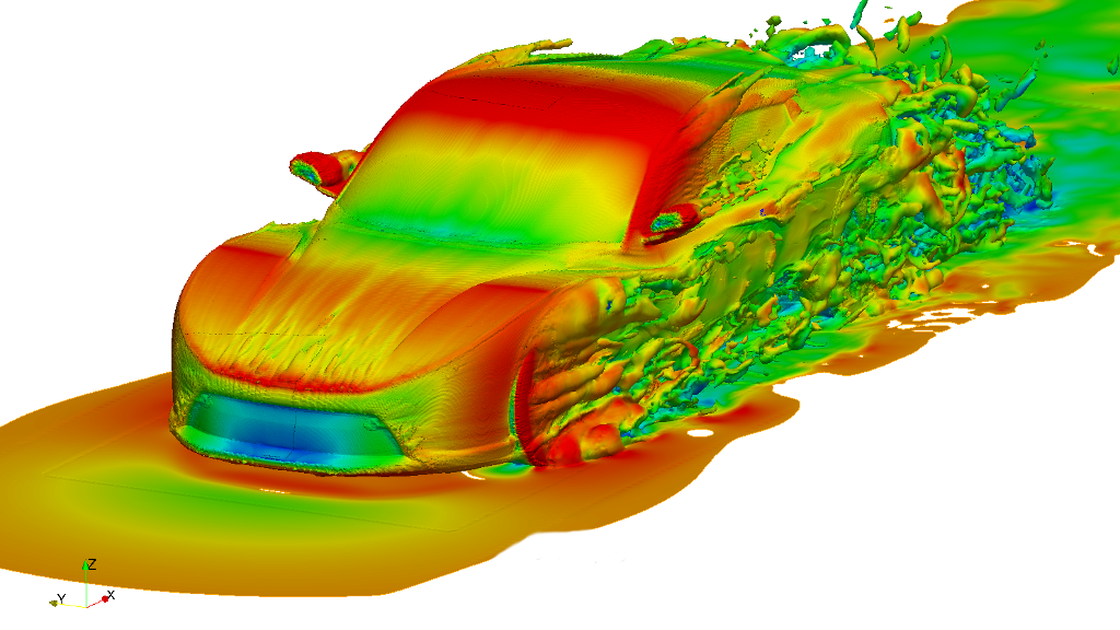 CFD is used to solve aerodynamics for vehicle. Image Source
Introduction
The project focuses on creating a numrical solver to solve the lid-driven cavity flow. In this problem, the side and bottom walls (boundaries) surrounding the cavity are fixed but the upper surface (lid) of the cavity is moved at a uniform velocity. Applications of lid driven cavities includes material processing, dynamics of lakes, metal casting and galvanizing. In this work, staggered grid was implemented to couple velocity and pressure and solve lid-driven cavity flow problem. Runge-Kutta iteration method was used for time advancements. The results were compared with the data from the Ghia, et al. [1] and matched very well. This project aims to provide a CFD simulation study of incompressible viscous laminar flow in cavity flow using Python.
Problem description
The cavity flow problem is described in the following figure. Basically, there is a constant velocity across the
top of the cavity which creates a circulating flow inside as shown in Fig 1. To simulate this there is a constant
velocity boundary condition applied to the lid, while the other three walls obey the no slip condition. Different
Reynolds numbers give different results, so in this article Re=100, and Re=1000 were applied. At high Reynolds
numbers we expect to see secondary circulation zones forming in the corners of the cavity.
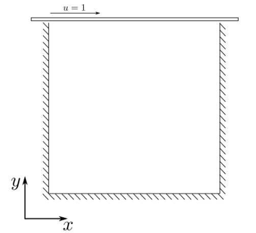 Physical description of lid-driven cavity flow.
Here is the system of differential equations(Navier-Stokes equations): two equations for the velocity
components u, v, and one equation for pressure p:
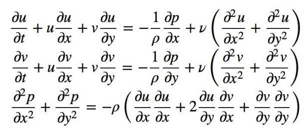 Navier-Stokes equations.
The initial condition is u,v,p=0; u,v,p=0 everywhere, and the boundary conditions are:
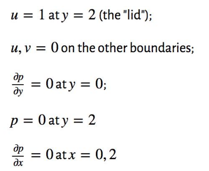 Boundary conditions of the problem
Methodology
In this article, projection method was applied to calculate fields. The projection method is an effective means of
numerically solving time-dependent incompressible fluid-flow problems. It was originally introduced by
Alexandre Chorin in 1967 [2] as an efficient means of solving the incompressible Navier-Stokes equations. The
key advantage of the projection method is that the computations of the velocity and the pressure fields are
decoupled. The basics of staggered grid can be illustrated in the figure below.
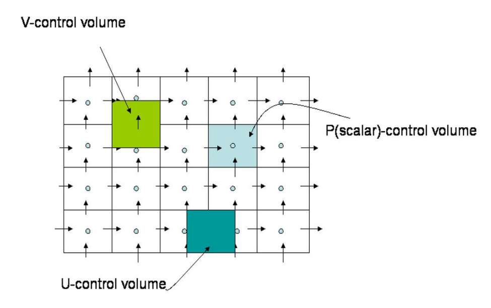 Staggered grid method.
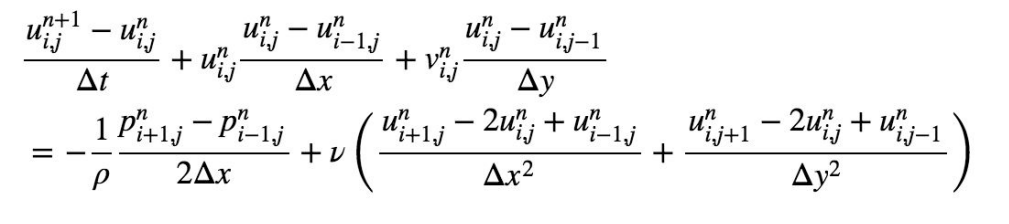
For u-momentum equation, discretization was as follows:
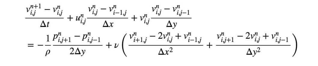
Similarly for the v-momentum equation:
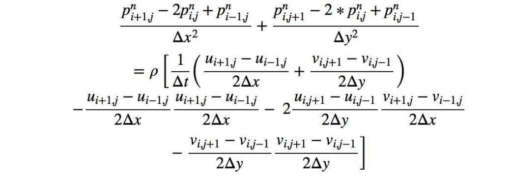
Finally, the discretized pressure-Poisson equation can be written as:
Results and Validation
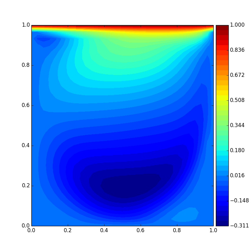
The contour plots for u, v, and p for Re = 100 and Re = 1000 were made to show the characteristics of the cavity
flow. Re = 100 was taken for low Reynolds number. The results were shown in below:
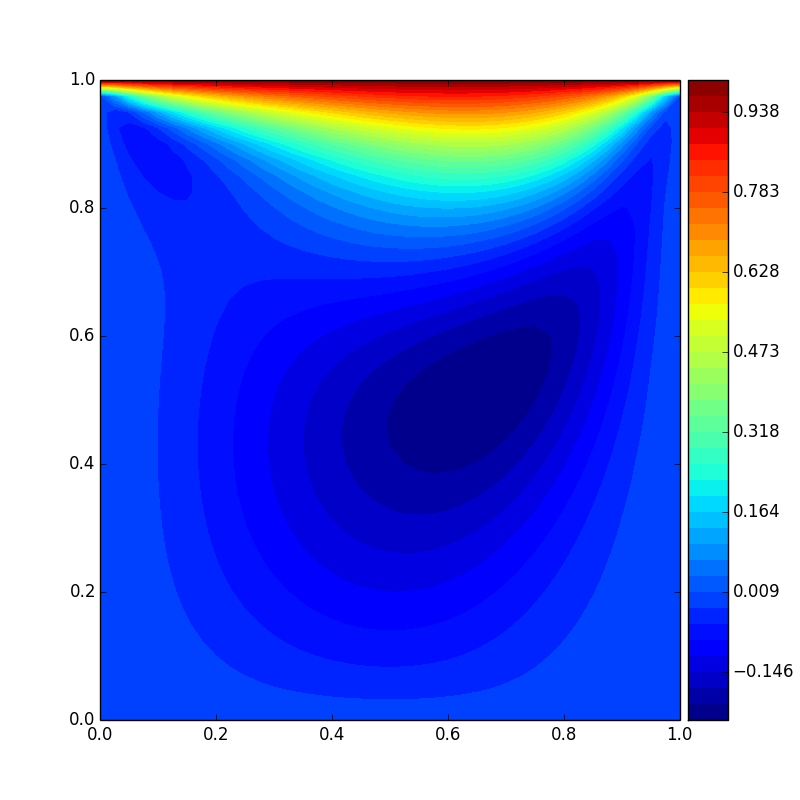 Horizontal velocity(Re = 100)
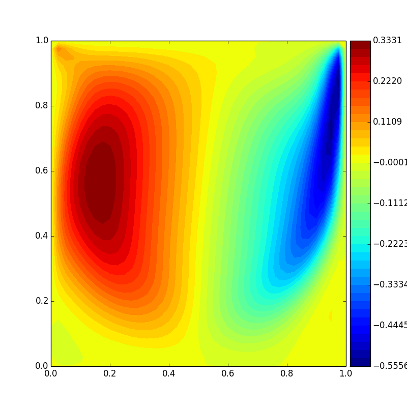
Vertical velocity(Re = 100)
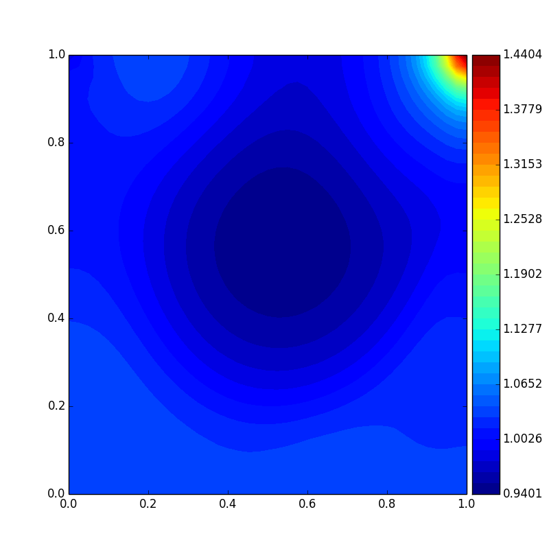
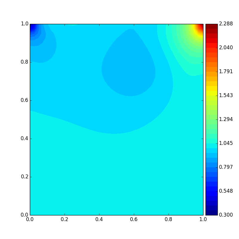 Pressure distribution(Re = 100)
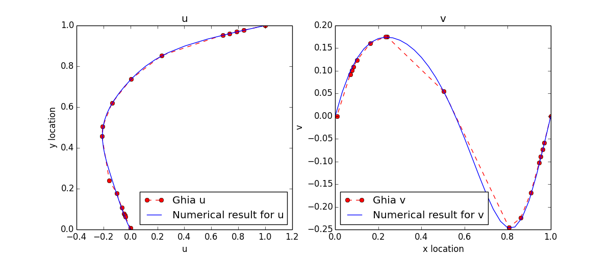
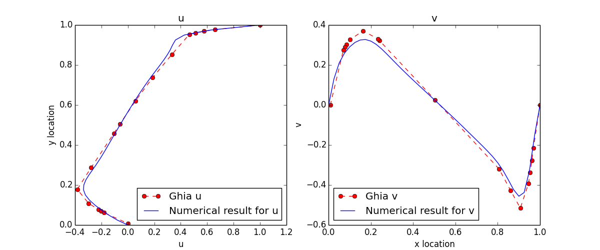
The simulation results match to the data points from Ghia, et al[1], very well:
Re = 1000 was taken for high Reynolds number. The results were shown below:
 Horizontal velocity(Re = 1000)
 Vertical velocity(Re = 1000)
 Pressure distribution(Re = 1000)
The simulation results also match to the data points from Ghia, et al[1], very well:
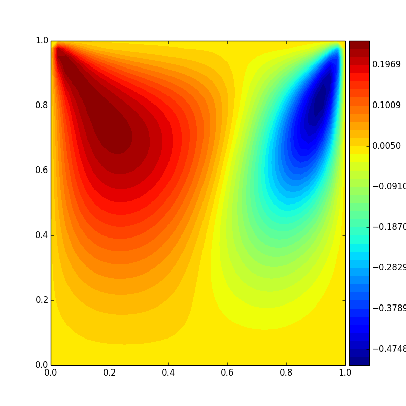
The contour plots for stream function and streamline plots for Re = 100 and Re = 1000 were made to show the
characteristics of the cavity flow in figures below:
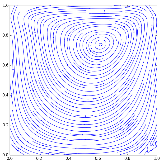 Streamlines contour plot(Re=100)
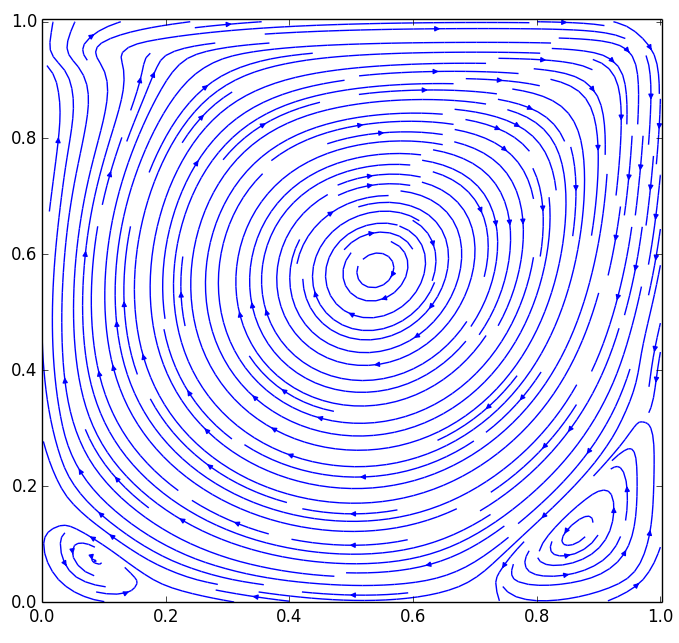 Streamlines contour plot(Re=1000)
Streamlines from Botella & Peyret (1998) [4]
In the comparison of u and v value along centerlines, the data matches to each other well except for the peak
value. This might happen when Reynolds number is high enough to bring error in.
Stream function from numerical simulation and stream function contour from Botella & Peyret (1998)[4] match
to each other quantitatively . The largest value is around 0.11(deep blue area) and
the lowest value is almost zero(deep red area). There are two areas on the two bottom corners where the stream
function value is a little bit above zero. This is caused by the secondary flows due to high Reynolds number for
this case.
Discussion and conclusions
In this work, numerical solutions with staggered grid and fully explicit time discretization were obtained for
laminar flow inside a square cavity of which lid moves at variable velocity and analytical solution is known (
Ghia, et al, 1982 and Botella & Peyret, 1998). The authors use a vorticity-stream function formulation of the 2D
N-S Momentum Equations with a coupled strongly implicit multigrid method.
Velocify field was plotted along centerlines. Results were also presented in the way of colorful contour plots to
compare with the existed publications.
This project was the summary of what was learnt in this course during this semester. We started with the 1-D
spatial discretization and moved toward the more complicated problems such as pressure Poisson equation
solver and parallel computation implementation on CFD. The last homework was particularly helpful in finding
the solutions of this project which introduces the ideas about how to code with Navier-Stokes equations. This
project closely resemble actual engineering problems and thus an important aspect of ME 614 Computational
Fluid Dynamics.
References
[1] Ghia, U. K. N. G., Ghia, K. N., & Shin, C. T. (1982). High-Re solutions for incompressible flow using the
Navier-Stokes equations and a multigrid method. Journal of computational physics, 48(3), 387-411.
[2]Chorin, A. J. (1967). The numerical solution of the Navier-Stokes equations for an incompressible fluid.
Bulletin of the American Mathematical Society, 73(6), 928-931.
[3] Babarinsa, O., Ogedengbe, E. O., & Rosen, M. A. (2014). Mixing Performance of a Suspended Stirrer for
Homogenizing Biodegradable Food Waste from Eatery Centers. Sustainability, 6(9), 5554-5565.
[4] Botella, O., & Peyret, R. (1998). Benchmark spectral results on the lid-driven cavity flow. Computers &
Fluids, 27(4), 421-433.